Introduction
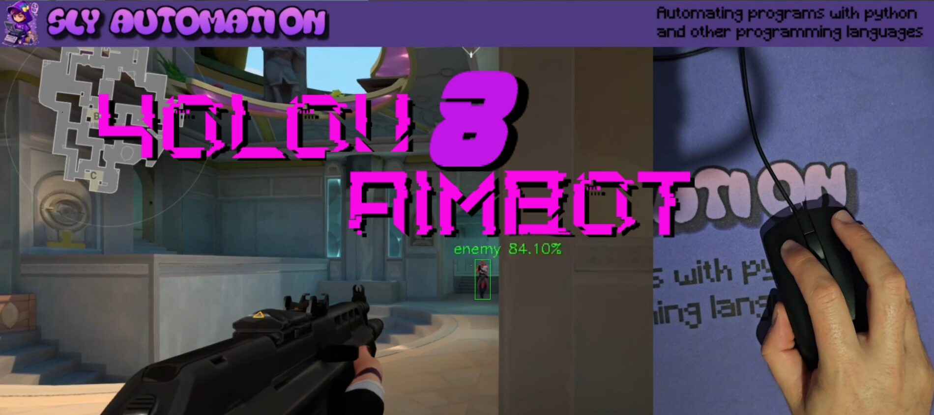
Greetings, fellow enthusiasts of computer vision and object detection, This is slyautomation and I am thrilled to welcome you to this in-depth tutorial where we will unravel the intricacies of training an aimbot using the cutting-edge YOLOv8. In this journey, I will be your guide, walking you through each step with clarity and precision.
Object detection is a fundamental task in computer vision, allowing machines to identify and locate objects within images or videos and with this we can use it for aimbotting. YOLOv8, short for “You Only Look Once version 8,” represents the latest iteration of this powerful object detection algorithm. Developed for speed and accuracy, YOLOv8 has become a go-to choice for researchers, developers, and enthusiasts in the field.
Github source: https://github.com/slyautomation/yolov8
For this build i’ll be using pycharm and cloning the github source for help see here: Install Pycharm and Python: Clone a github project
💥🎯 Just want the sweet juicy yolov8 aimbot steps install, download model and run! 🚀✨
- Installs (cuda & cudnn, pip installs)
- Data (use this to train your own aimbot for fortnite, pubg or apex!)
- Models (apex, pubg, fortnite)
- Run!
Contents
- The Significance of YOLOv8
- Step 1: Data Collection
- 1.1 Selecting a Dataset or Gathering Your Own
- 1.2 Downloading or Capturing Game Object Images
The Significance of YOLOv8
Why choose YOLOv8? Its significance lies not only in its state-of-the-art performance but also in its efficiency. YOLOv8 can detect objects in real-time, making it suitable for applications ranging from surveillance and autonomous vehicles to wildlife monitoring and beyond. With the ability to process images rapidly and accurately, YOLOv8 has become a cornerstone in the realm of computer vision and is the latest version as at 2024!
So, without further ado, let’s embark on this exciting adventure into the world of YOLOv8 and custom object detection!
Nvidia Cuda Install
Ready to supercharge your YOLOv8 experience? Dive into the world of GPU acceleration with CUDA, the secret sauce behind lightning-fast object detection! 🚀💡
Discover the Game-Changing Steps to Install CUDA for YOLOv8:
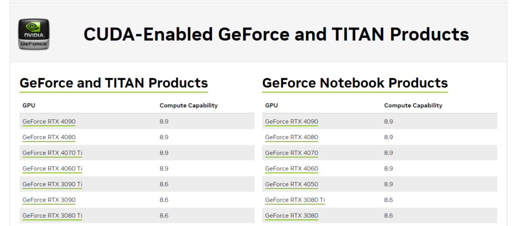
🔍 Check GPU Compatibility: Ensure your GPU is a perfect match for the CUDA version you’re about to unleash! Find all the deets on the Nvidia website. 🕵️♂️💻 https://developer.nvidia.com/cuda-gpus Use this to lookup your GPU:
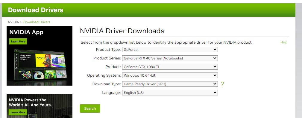
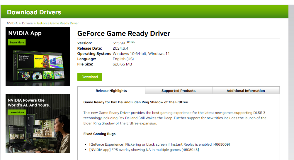
🔧 Install Nvidia GPU Drivers: Before you embark on your CUDA journey, gear up with the latest Nvidia GPU drivers tailored for your graphics card. Get them straight from the Nvidia website! 🚗💨🔥 https://www.nvidia.com/download/index.aspx Add your GPU specs, then click search!
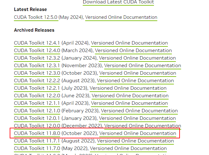
🚀 Install CUDA Toolkit GET 11.8!!!: Grab the power-packed CUDA Toolkit version from Nvidia, perfectly tuned for YOLOv8 compatibility with PyTorch. Follow Nvidia’s installation magic for a seamless setup! 🌐💻 https://developer.nvidia.com/cuda-toolkit-archive
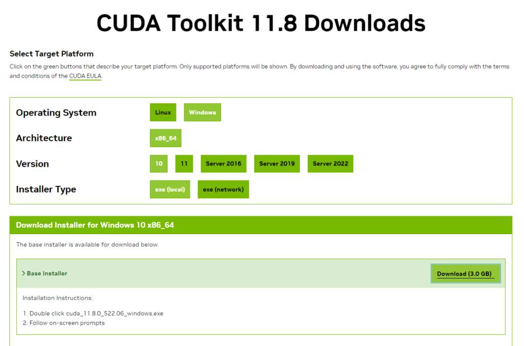
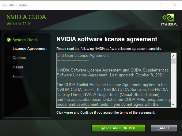
Once downloaded click the file to download and begin installation.
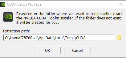
Use the standard options on the installation prompts!
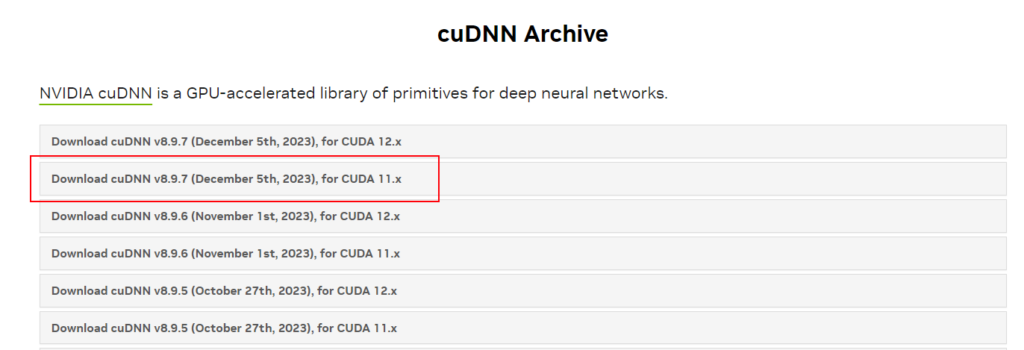
🔥 Install cuDNN GET FOR 11.X!!!: Unleash the full potential with the cuDNN library! Download the version that syncs with your CUDA version, extract the magic, and seamlessly integrate it into your CUDA Toolkit haven. 📥✨💼 https://developer.nvidia.com/rdp/cudnn-archive (Download whatever once is the latest dated version of 11.X)
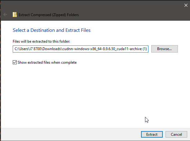
CuDNN Install Steps:
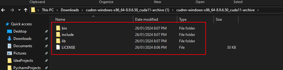
Extract the zip file just downloaded for cuDNN:
Copy contents including folders:
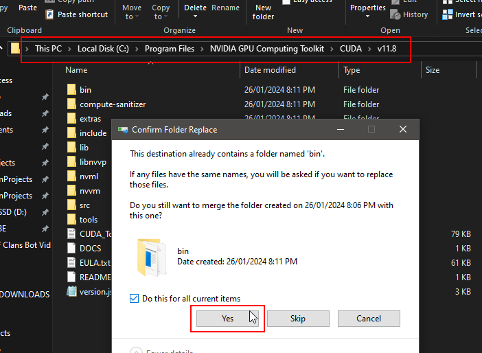
Locate NVIDIA GPU Computing Toolkit folder and the CUDA folder version (v11.8) and paste contents inside folder:
Ready to elevate your YOLOv8 game? Follow these steps, and let the CUDA adventure begin! 🚀💥 #YOLOv8 #CUDAInstallation #TechMagic”
Step 1: Data Collection
Data collection serves as the foundation for any successful machine learning project, and object detection with YOLOv8 is no exception. In this step, we’ll delve into the intricacies of acquiring a diverse and representative dataset for our enemies for a fortnite aimbot object detection task.
1.1 Selecting a Dataset or Gathering Your Own
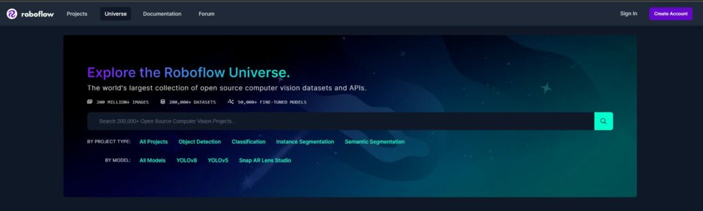
The first decision you need to make is whether you’ll be using an existing dataset or creating your own. Existing datasets can be advantageous, especially for already established objects in the aimbotting space like apex, fortnite and counter strike. Websites such as Kaggle, ImageNet, Roboflow or other dedicated dataset repositories can provide suitable options. However, for more specialized tasks, like detecting in a niche game, you might need to gather your own data.
1.2 Downloading or Capturing Game Object Images
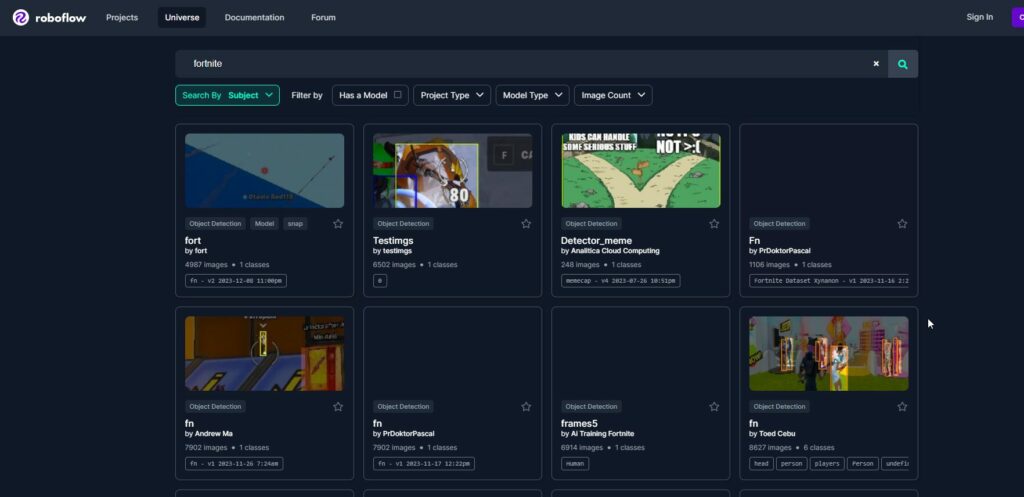
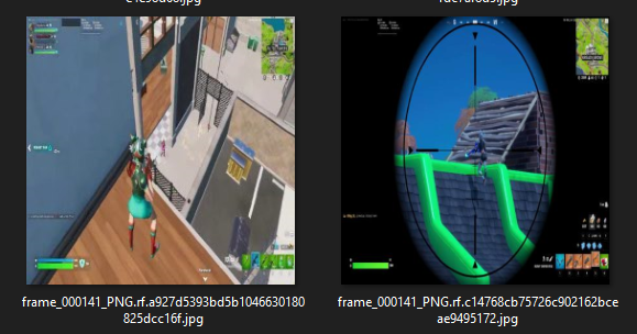
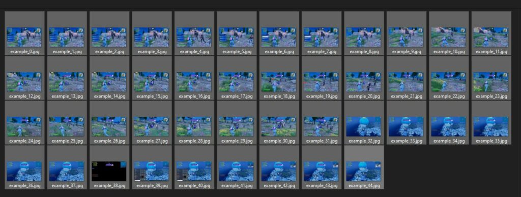
In our case, we’ve opted for a dataset featuring enemies in fortnite for a fortnite aimbot. I’ve downloaded a set of images showcasing enemies in fortnite from roboflow. When selecting or capturing images, aim for diversity in backgrounds, lighting conditions, and fortnite enemies orientations. This diversity helps the model generalize well to different scenarios.
1.3 Organizing and Managing Your Dataset
Once you have your images, it’s crucial to organize them systematically. Consider creating folders for training, validation, and testing sets.
datasets
├─ apex
├─ fortnite
│  ├─ images
│  ├─ labels
│  ├─ valid
├─ titanfall
│  ├─ images
│  ├─ labels
├─ counterstrike
├─ pubg
├─ cod
A well-organized dataset simplifies the subsequent annotation and training processes. Additionally, label your images with meaningful filenames or folder structures to keep track of different classes or categories.
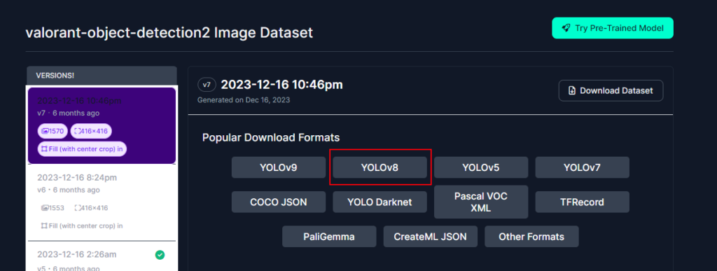
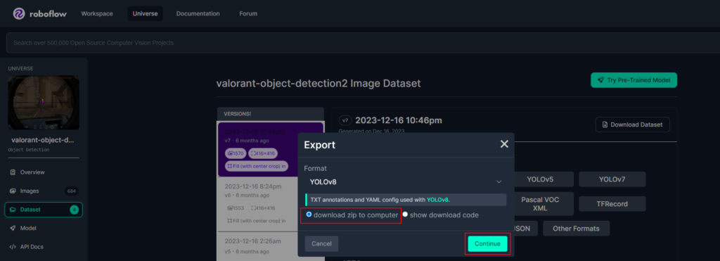
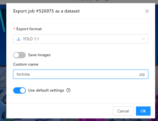
With Roboflow, you can download a dataset that is automatically formatted to yolov8! Make sure to select the option ‘YOLOv8’ and select download zip to computer.
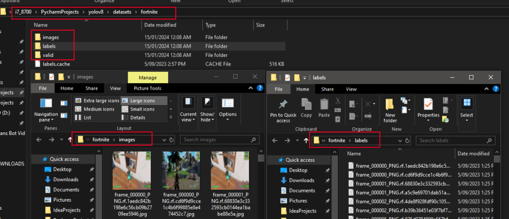
save you dataset to your yolov8 project directory in ‘datasets’!
1.4 Dataset Size and Balance
The size of your dataset matters. While more data generally leads to better models, ensure a balance between sufficiency and avoiding redundancy. A dataset that adequately represents the real-world scenarios your model will encounter is key to achieving robust and reliable performance.
1.5 Data Augmentation
To enhance model generalization and prevent overfitting, consider applying data augmentation techniques. These may include random rotations, flips, or changes in lighting conditions. Data augmentation helps the model adapt to a wider range of scenarios than those present in the original dataset.
1.6 Dataset Licensing and Ethics
Always be mindful of the licensing agreements associated with the datasets you use and adhere to ethical considerations. If you’re capturing your own images, respect privacy and ensure proper consent. Ethical data practices contribute to the responsible development of machine learning models.
In conclusion, Step 1 is about laying the groundwork for success. Whether you choose an existing dataset or collect your own, thoughtful consideration in dataset selection and organization will greatly impact the overall effectiveness of your YOLOv8 object detection model. Now that our dataset is ready, we can proceed to Step 2: Data Annotation.
Step 2: Data Annotation – Precise Marking of Fortnite Enemies for the aimbot
Data annotation is a critical step in the process of training an object detector, as it involves marking and labelling objects of interest in the images. In our case, we are focusing on annotating images featuring enemies for a fortnite aimbot using a computer vision annotation tool. Let’s delve deeper into this crucial step:
2.1 Choosing the Right Annotation Tool
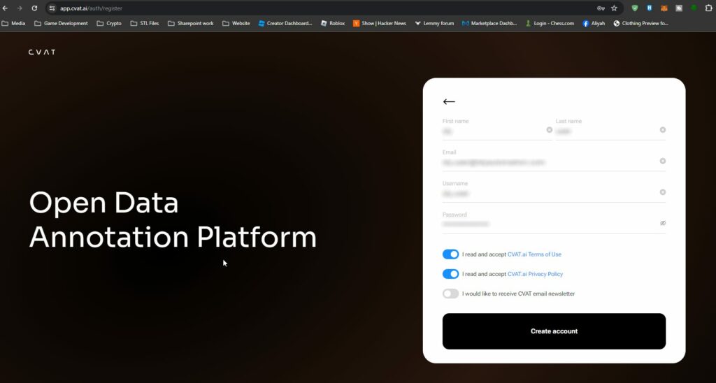
Selecting an appropriate annotation tool is essential. Tools like CVAT (Computer Vision Annotation Tool) provide a user-friendly interface for annotating objects in images. In this tutorial, we’ll use CVAT for its versatility and ease of use. For a more detailed step by step guide on using cvat.ai and data annotation go here: CVAT – Computer Vision Annotation Tool – Open Data Annotation Platform for Image & Video
2.2 Creating a Project and Adding Labels
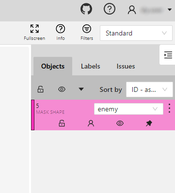
Once logged into the annotation tool, the first step is to create a new project. In our case, we’ll name it “Fornite Aimbot Enemies”. Within the project, we upload the images, we add a label config corresponding to the object we want to detect, which is “enemy” in this scenario. This step is crucial, as it sets the groundwork for labelling instances of enemies in the images.
2.3 Image Annotation
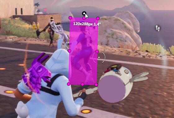
With the project and label set up, we can proceed to annotate individual images. Using the annotation tool, we select the object label (“enemy”) and draw bounding boxes around each fornite enemy in the image. The goal is to encapsulate the enemy within the bounding box accurately so the fornite aimbot recognises the whole element of th object.
2.4 Handling Varied Poses and Situations
It’s important to note that images in the dataset may feature alpacas in various poses and situations. The annotator’s task is to identify and annotate fortnite enemies irrespective of their positions, ensuring comprehensive coverage. You may encounter challenges such as reflections, partial views, or diverse postures, requiring a keen eye for detail and multiple enemies in one image, be sure to annote them all!.
2.5 Consistency in Annotation
Consistency is key during annotation for the fortnite aimbot. Annotators should follow a standardized approach, drawing bounding boxes around fortnite enemies in a consistent manner. This uniformity ensures that the model learns effectively from the annotated data.
2.7 Saving Annotations
After annotating a set of images, the annotations need to be saved.
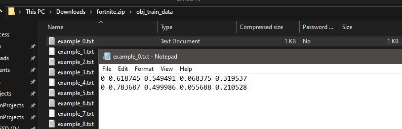
In CVAT, for example, the annotations can be exported in various formats, including the YOLO format required for training YOLOv8. This format typically includes the class ID, the position of the bounding box centre, and the width and height of the bounding box.
By the end of the annotation process, each image in the dataset should have accurate and consistent bounding box annotations around alpacas, forming the foundation for effective machine learning model training.
Remember, the quality of annotations directly influences the model’s ability to recognize and detect objects accurately during the training phase. Careful and meticulous annotation ensures a robust dataset, paving the way for successful object detection model training.
Step 3: Data Structuring
Once we’ve annotated our dataset, the next crucial step is to structure the data in a way that YOLOv8 can effectively utilize it for training. Proper organization ensures that the model can seamlessly understand and learn from the data. In this step, I’ll guide you through the process of organizing your annotated dataset.
If you used cvat.ai the data structure and label files for the directory heirarchy will already be provided!
Image and Annotation Directories:
Create Directory Hierarchy:
- Consider creating separate directories for training and validation datasets to facilitate the model’s performance evaluation. This can be achieved by having two directories like train and validation.
├── images
│   ├── train
│   │   ├── image1.jpg
│   │   ├── image2.jpg
│   │   └── ...
│   └── validation
│       ├── image1.jpg
│       ├── image2.jpg
│       └── ...
└── labels
    ├── train
    │   ├── image1.txt
    │   ├── image2.txt
    │   └── ...
    └── validation
        ├── image1.txt
        ├── image2.txt
        └── ...
Here, the images directory contains subdirectories for both training and validation datasets. The corresponding labels directory follows the same structure.
Label Files in YOLO Format:
- Each image in the dataset must have a corresponding label file in YOLO format. YOLO format represents object coordinates in the image and is usually a text file with the same name as the image but with a .txt extension.
# Example of YOLO annotation format for a single object in an image
class_id center_x center_y width height- For instance, if your image is image1.jpg, the corresponding label file will be image1.txt.
YAML Configuration File:
Create a YAML Configuration File:
- Generate a YAML file to configure the training process. This file, commonly named your_dataset.yaml, will contain essential information such as paths to your datasets, model configuration, and training parameters.
# Example YAML Configuration File
train_path: 'images/train'
val_path: 'images/validation'
num_classes: 1
# ... other configuration parameters- Make sure to specify the paths relative to the location of your YAML file.
Configure Class Information:
- Indicate the number of classes your model is detecting. In the example above, num_classes is set to 1 as we are detecting enemies.
Summary:
Proper data structuring involves creating a well-organized directory hierarchy and configuring a YAML file to guide the training process. YOLOv8 relies on these structures to efficiently train and learn from your annotated data. Ensure that paths in the YAML file accurately reflect the location of your dataset directories, and you’re ready to move on to the exciting training phase in Step 4!
Step 4: Training with YOLOv8
Now that we’ve prepared our annotated dataset, it’s time to move on to the heart of the process – training our YOLOv8 model. Training involves teaching the model to recognize patterns and features in the data, enabling it to accurately detect objects in new, unseen images.
In the context of training a YOLO (You Only Look Once) model, adjusting the batch size and the number of epochs are important hyperparameters that can impact the training process and the performance of the model. Here’s how changing these parameters can be useful:
- Batch Size:
- Impact on Training Speed: The batch size represents the number of samples that are processed in a single iteration during training. A larger batch size can lead to faster training as more data is processed in parallel. However, it may require more memory, and very large batch sizes can sometimes lead to convergence issues.
- Regularization Effect: Smaller batch sizes introduce more noise into the training process, which can act as a form of regularization. This regularization effect might help the model generalize better to unseen data.
- GPU Memory Constraints: The choice of batch size is often constrained by the available GPU memory. If you have a powerful GPU with large memory, you can experiment with larger batch sizes.
- Epochs:
- Number of Training Iterations: An epoch is one complete pass through the entire training dataset. Increasing the number of epochs allows the model to see the entire dataset multiple times, potentially improving performance. However, too many epochs can lead to overfitting.
- Early Stopping: Monitoring the model’s performance on a validation set during training can help decide when to stop training. If the performance stops improving or starts to degrade on the validation set, training can be stopped early to prevent overfitting.
- Learning Rate Scheduling: The number of epochs is often related to learning rate scheduling. Learning rates may need to be adjusted during training, and the number of epochs influences when and how these adjustments occur.
It’s important to note that the optimal values for batch size and the number of epochs can depend on the specific dataset, model architecture, and other hyperparameters. It’s common practice to experiment with different values and monitor the model’s performance on a validation set to find the best combination for your specific task. Additionally, techniques like learning rate annealing, data augmentation, and transfer learning can also impact training dynamics and model performance.
4.0 Setting up your project with the required modules and software to run Yolov8
Install Dependencies: Make sure you have Python and pip installed on your system. Preferably use a IDE such as Pycharm, Spyder or Juypter Notebooks and create a virtual environment if desired. Need a guide on setting up Pycharm? Got you covered! Install Pycharm and Python: Clone a github project
Then follow these steps to get the project ready for training on yolov8:
# Install the ultralytics package from PyPI
pip install ultralytics
So it’s recommended to install PyTorch using the instructions here at https://pytorch.org/get-started/locally. The interactive page wil help you determine the install command based on your os and pc requirements.
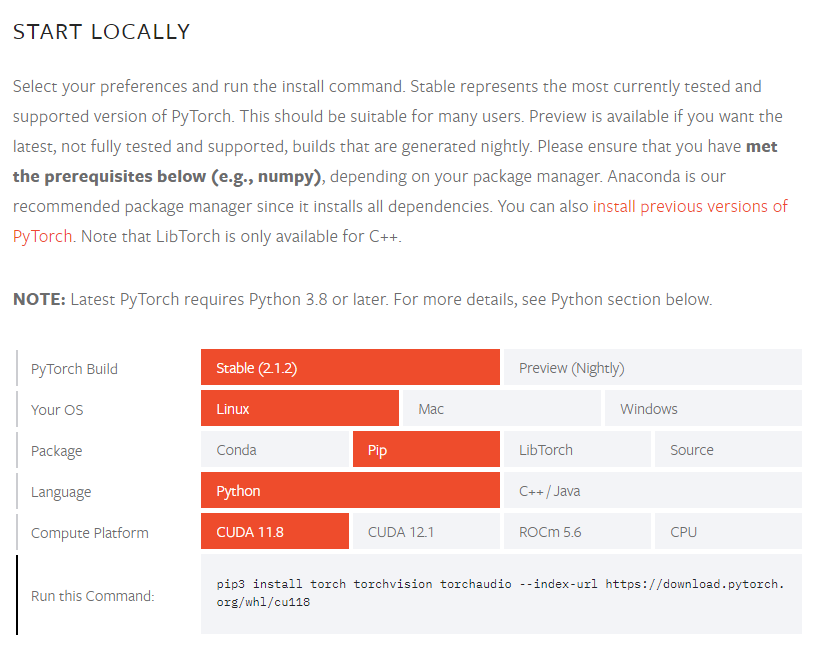
As shown in the above image i need to run the command:
pip3 install torch torchvision torchaudio --index-url https://download.pytorch.org/whl/cu118If this causes issues i find the following command works:
pip install --upgrade --force-reinstall torch torchvision torchaudio --index-url https://download.pytorch.org/whl/cu118🚀 Unleash the Power of PyTorch: Verify Your Installation in Minutes! 🚀
👉 Dive into the PyTorch Universe with Confidence! Let’s confirm your PyTorch installation in a heartbeat:
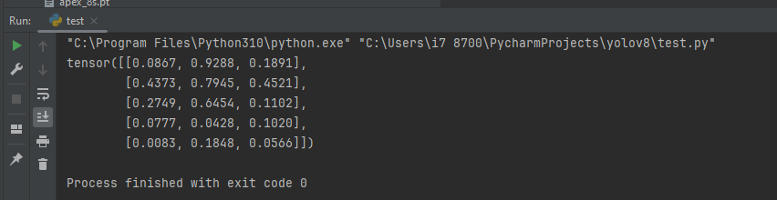
- 🔍 Sample Code Check: Run this magical PyTorch code to ensure your installation is as smooth as butter!
import torch
x = torch.rand(5, 3)
print(x)
🎉 Your screen should light up with a dazzling tensor like:
💥 GPU Verification Blitz: Supercharge your PyTorch experience by ensuring your GPU driver and CUDA/ROCm are ready for action! Execute these commands to unveil the GPU magic. This should return True.
import torch
print(torch.cuda.is_available())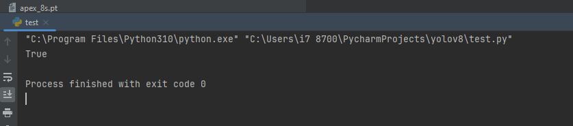
4.1 Choosing the YOLOv8 Variant
Before we delve into training, it’s essential to choose the YOLOv8 variant that suits your project’s requirements. YOLOv8 comes in various sizes, from the lightest Nano version to larger models with more parameters. In the tutorial, we opt for the standard YOLOv8 S, the 2nd smallest model that strikes a balance between speed and accuracy.
| Model | size (pixels) | mAPval 50-95 | Speed CPU ONNX (ms) | Speed A100 TensorRT (ms) | params (M) | FLOPs (B) |
|---|---|---|---|---|---|---|
| YOLOv8n | 640 | 37.3 | 80.4 | 0.99 | 3.2 | 8.7 |
| YOLOv8s | 640 | 44.9 | 128.4 | 1.20 | 11.2 | 28.6 |
| YOLOv8m | 640 | 50.2 | 234.7 | 1.83 | 25.9 | 78.9 |
| YOLOv8l | 640 | 52.9 | 375.2 | 2.39 | 43.7 | 165.2 |
| YOLOv8x | 640 | 53.9 | 479.1 | 3.53 | 68.2 | 257.8 |
- mAPval values are for single-model single-scale on COCO val2017 dataset.
Reproduce byyolo val detect data=coco.yaml device=0 - Speed averaged over COCO val images using an Amazon EC2 P4d instance.
Reproduce byyolo val detect data=coco.yaml batch=1 device=0|cpu
4.2 Parameters and Configuration File (config.yaml)
To initiate the training process, we need to use the configuration file, as created above named your_dataset.yaml. This file contains crucial information about the dataset and the number of classes.
To train a YOLOv8 model, you can use the main.py file and use the custom_train function. By default, it loads the COCO dataset configuration (coco128.yaml). This function is responsible for training a YOLOv8 model. It takes several parameters:
load: Specifies the model initialization strategy. Use ‘new’ to build a new model, ‘pre’ to load a pretrained model, and ‘tran’ to build from YAML and transfer weights.traindata: YAML file specifying the training data configuration.epoch: Number of training epochs.batc: Batch size for training.export: IfTrue, exports the trained model to ONNX format.val: IfTrue, prints and returns metrics after validation.
Here, we specify the image size, batch size, number of epochs, the path to the configuration file, and pre-trained weights (optional).
custom_train(load='pre', traindata="coco128.yaml", epoch=50, batc=3, export=False, val=True)run_checks Function
This function checks the model detection is still using the GPU for cuda computing.
def run_checks():
  ultralytics.checks()
  print("Using GPU:", torch.cuda.is_available())
predict Function
This function performs inference using a trained YOLOv8 model. It takes the following parameters:
def predict(mod='best.pt', sourc='screen', sav=True, sho=False,  imgs=(800,800), con=0.3, save_tx=False):
    model = YOLO(mod)
model.predict(source=sourc, save=sav, show=sho, imgsz=imgs, conf=con, save_txt=save_tx)- mod: Load a pretrained YOLOv8 model ‘yolov8n.pt’, ‘yolov8n.pt’, ‘yolov8s.pt’, ‘yolov8m.pt’, ‘yolov8l.pt’, ‘yolov8x.pt’ or custom ‘best.pt’ etc.
sourc: Source of inference. Options include ‘screen’ for screenshots, ‘image.jpg’ for image file, or ‘video.mp4’ for video file.sav: IfTrue, saves the predictions.sho: IfTrue, displays the predictions.imgs: Tuple specifying the input image size.con: Confidence threshold for predictions.save_tx: IfTrue, saves predictions as labels.
There’s more that can be done for more information go here: https://docs.ultralytics.com/modes/predict/
The __main__ block at the end of the script demonstrates a typical workflow. It runs checks, trains a model with custom settings, loads a pretrained model, and performs prediction on an example image.
if __name__ == '__main__':
    run_checks()
    custom_train(traindata="osrs.yaml")
    model.predict(mod='best.pt', sourc='bus.jpg', save=True, show=True, imgsz=320, conf=0.5)
    predict()
The functions that are not required can be commented out when running the python file. Remember to adjust the parameters based on your specific use case and data. Additionally, make sure to have the necessary data configuration files (e.g., YAML files).
Ultralytics will automatically handle the downloading of YOLOv8 models, making the process more straightforward.
4.3 Training from a Local Environment
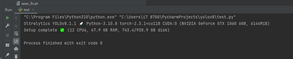
Then lets check yolov8 is installed!
from IPython import display
display.clear_output()

import ultralytics
ultralytics.checks()
be sure to change main.py and change the value in traindata to the desired yaml file too:
if __name__ == '__main__':
run_checks()
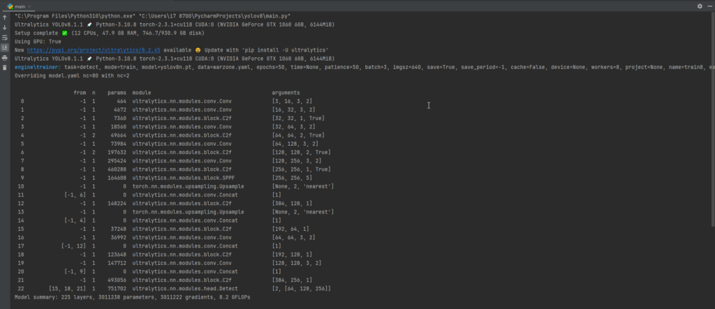
custom_train(traindata="valorant.yaml")If you prefer working in your local environment, using tools like PyCharm or Jupyter notebooks, you can initiate training from the command line. By executing a command like:
# Be sure to make your parameters changes in the main.py file
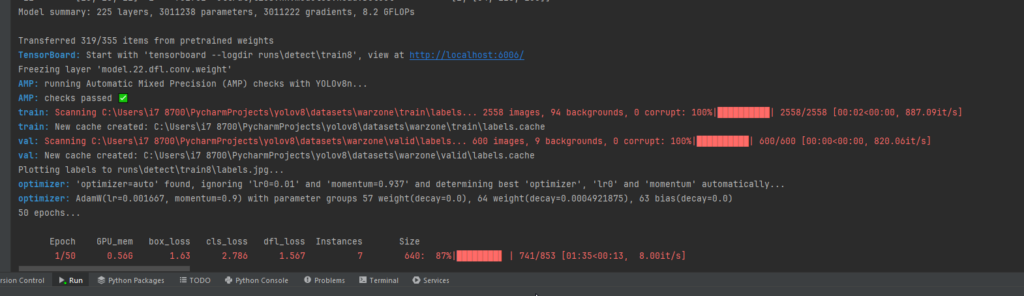
python main.py4.5 Monitoring Training Progress
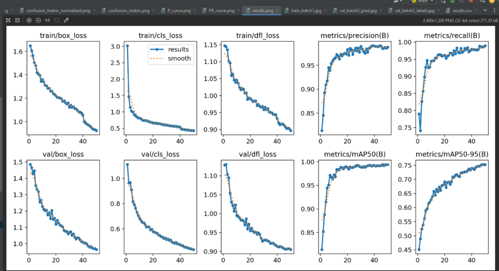
Throughout the training process, YOLOv8 provides real-time updates on various metrics like loss, precision, recall, and more. These metrics are essential for gauging how well the model is learning from the data. You’ll observe plots, generated and saved in designated directories, that visually represent the training progress.
4.6 Saving and Analyzing Results
After training concludes, YOLOv8 saves the model weights and additional information, such as training curves and other performance metrics, in specific directories. Analyzing these results can provide insights into how well the model has learned from the data.
Conclusion of Step 4
By following these steps, you’ll have successfully trained a YOLOv8 model on your custom dataset. Whether you opt for a local environment or leverage the convenience of Google Colab, the training process remains intuitive and accessible. Now, armed with a trained model, it’s time to move on to the final step – testing and evaluating the model’s performance.
Step 5: Testing and Performance Evaluation
After the intensive training process, it’s time to assess how well our YOLOv8 model performs on real-world data. This step involves testing the model on images and videos to evaluate its accuracy and efficiency in detecting alpacas. Let’s delve deeper into this crucial phase of the object detection pipeline.
5.1 Model Inference on Images
We’ll start by performing inference on a set of test images. Using the trained YOLOv8 model, we’ll detect alpacas in these images and visualize the results. This step helps us visually inspect the model’s predictions and identify any potential issues, such as false positives or misses.
5.2 Evaluation Metrics
To quantify the model’s performance, we’ll introduce key evaluation metrics commonly used in object detection tasks. These metrics include precision, recall, and the F1 score. Understanding these metrics is essential for objectively assessing the model’s ability to correctly identify alpacas while minimizing false alarms. These metrics are available in the ‘runs’ folder in the trainxx folder. Here’s an example after a trained model on Valorant was completed
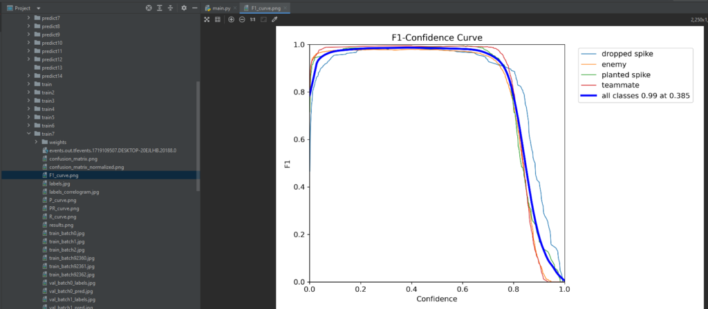
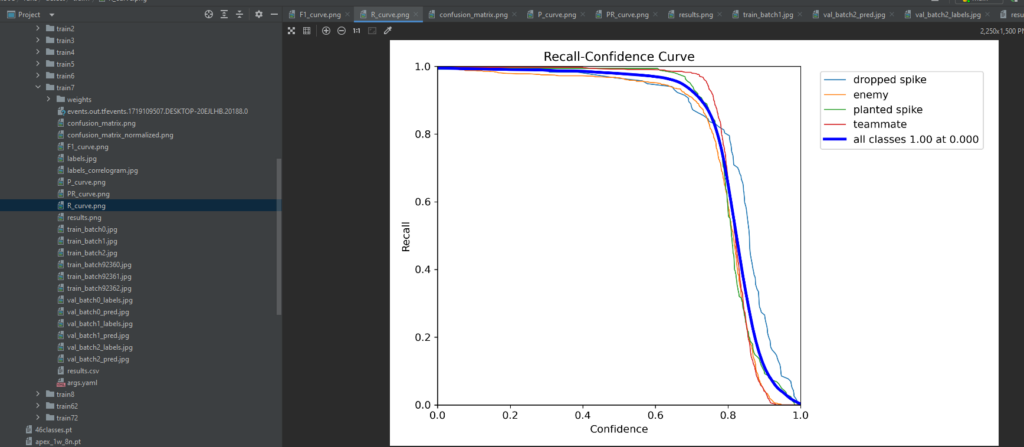
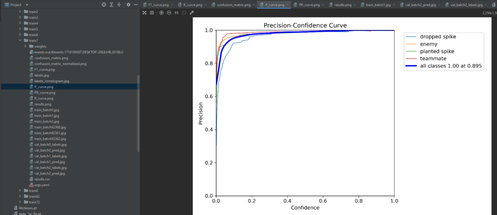
5.3 Visualization of Metrics
We won’t just stop at calculating metrics – we’ll visualize them to gain deeper insights. Graphs and charts depicting precision-recall curves or confusion matrices will provide a comprehensive overview of the model’s strengths and weaknesses. This visualization step aids in making informed decisions about potential improvements or adjustments to the training process. These metrics are available in the ‘runs’ folder in the trainxx folder and can be accessed by viewing the result.png which has all the data to analyze the results of training the model.
Conclusion of Step 5
The testing and performance evaluation step is critical in determining the practical utility of our YOLOv8 model. By the end of this phase, you’ll have a comprehensive understanding of how well the model generalizes to new data and be equipped to make informed decisions on potential optimizations or improvements. This step marks the bridge between model development and its real-world applicability, bringing your object detection project to a satisfying conclusion.
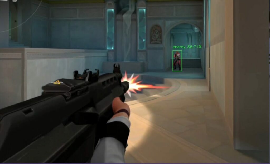
Viewing the aimbot results
Run the file view_aimbot.py to have a view only mode of the aimbot to see if it works. This will loop through screenshots of the display monitor while you the user plays the game!
Parsing Predictions
    boxes_data = []
    for result in predictions:
        boxes = result.boxes
        for box in boxes:
            b = box.xyxy[0]  # get box coordinates in (left, top, right, bottom) format
            c = box.cls
            conf = box.conf[0]  # Get confidence score
            label = f"{model.names[int(c)]} {conf*100:.2f}%"
            boxes_data.append((b, label))
    return boxes_data
- boxes_data: An empty list to store bounding box coordinates and labels.
- result.boxes: Contains bounding boxes for detected objects.
- box.xyxy[0]: Retrieves coordinates of the bounding box in the format
(left, top, right, bottom). - box.cls: Class index of the detected object.
- box.conf[0]: Confidence score of the detection.
- label: Formatted string with the object name and confidence percentage.
- boxes_data.append((b, label)): Appends the bounding box coordinates and label to the list.
- return boxes_data: Returns the list of bounding boxes and labels.
Main Code Execution
Initialization
if __name__ == '__main__':
    osrs_monitor = {"top": 0, "left": 0, "width": 800, "height": 800}
    monitor = {"top": 0, "left": 0, "width": 1920, "height": 1080}
    sct = mss()
    mod = 'valorantv2.pt'
    model = YOLO(mod)
    Bot = True
- osrs_monitor: Dictionary defining the size and position of a smaller screen capture area.
- monitor: Dictionary defining the size and position of the full screen capture area.
- sct: Initializes the screen capture tool
mss. - mod: Specifies the YOLO model file.
- model: Loads the YOLO model.
- Bot: A boolean variable to control the main loop.
    while Bot:
        img = np.array(sct.grab(monitor))
        img = cv2.cvtColor(img, cv2.COLOR_BGRA2BGR)
        bigger = cv2.resize(img, (800, 800))
        boxes_data = custom_predict(sourc=bigger, sav=False, sho=False)
        for box, label in boxes_data:
            # Rescale the bounding box back to the original image size
            box = [int(coord * 1920 / 800) if i % 2 == 0 else int(coord * 1080 / 800) for i, coord in enumerate(box)]
            start_point = (box[0], box[1])
            end_point = (box[2], box[3])
            color = (0, 255, 0)
            thickness = 1
            img = cv2.rectangle(img, start_point, end_point, color, thickness)
            img = cv2.putText(img, label, (box[0], box[1] - 10), cv2.FONT_HERSHEY_SIMPLEX, 0.5, color, thickness)

        cv2.imshow("images", img)
        cv2.waitKey(5)
- img = np.array(sct.grab(monitor)): Captures the screen image as a NumPy array.
- img = cv2.cvtColor(img, cv2.COLOR_BGRA2BGR): Converts the image from BGRA to BGR color space.
- bigger = cv2.resize(img, (800, 800)): Resizes the image to (800, 800) for prediction.
- boxes_data = custom_predict(sourc=bigger, sav=False, sho=False): Gets bounding box predictions and labels from the resized image.
- for box, label in boxes_data: Iterates through each bounding box and label.
- box = [int(coord * 1920 / 800) if i % 2 == 0 else int(coord * 1080 / 800) for i, coord in enumerate(box)]: Rescales the bounding box coordinates back to the original image size.
- start_point = (box[0], box[1]): Top-left corner of the bounding box.
- end_point = (box[2], box[3]): Bottom-right corner of the bounding box.
- color = (0, 255, 0): Color of the bounding box (green).
- thickness = 1: Thickness of the bounding box lines.
- img = cv2.rectangle(img, start_point, end_point, color, thickness): Draws the bounding box on the original image.
- img = cv2.putText(img, label, (box[0], box[1] – 10), cv2.FONT_HERSHEY_SIMPLEX, 0.5, color, thickness): Puts the label text above the bounding box.
- cv2.imshow(“images”, img): Displays the annotated image in a window named “images”.
- cv2.waitKey(5): Waits for 5 milliseconds for a key press. This loop will keep running until interrupted.
Conclusion
Congratulations! You’ve just completed a comprehensive journey through the intricate process of training YOLOv8 on a custom dataset for object detection. As we wrap up this tutorial, let’s reflect on what you’ve achieved and discuss potential next steps in your computer vision endeavors.
Key Takeaways
Data is Key: The importance of a well-annotated and structured dataset cannot be overstated. The success of your object detection model is deeply intertwined with the quality and diversity of your training data.
Annotation Precision: You’ve learned the art of data annotation, emphasizing the precision required when drawing bounding boxes. Clear instructions and meticulous labeling lay the foundation for a robust model.
Configuration Mastery: Navigating the YOLOv8 configuration file is a skill you’ve honed. Understanding the paths, specifying directories, and fine-tuning hyperparameters are essential for a successful training process.
Training Strategies: Whether working in a local environment or utilizing Google Colab, you’ve witnessed the simplicity of initiating the training process. The careful evaluation of training metrics allows you to iterate and enhance model performance.
Testing and Performance Evaluation: The final step involved testing the trained model on new data. You’ve gained insights into interpreting performance metrics, allowing you to assess the model’s accuracy, recall, and precision.
Next Steps
Further Training: If your model’s performance leaves room for improvement, consider conducting additional training iterations. Experiment with different hyperparameters, increase the number of epochs, or explore more advanced training techniques.
Data Augmentation: Enhance your dataset by incorporating data augmentation techniques. This can include rotations, flips, and changes in lighting conditions, providing your model with a more comprehensive understanding of object variations.
Transfer Learning: Explore the possibilities of transfer learning by using pre-trained models. This approach can save time and resources while leveraging the knowledge gained from models trained on large, diverse datasets.
Fine-Tuning for Specific Use Cases: Tailor your model to specific use cases by fine-tuning on datasets relevant to your application. This ensures the adaptability of your object detection system to varying scenarios.
Community Engagement: The field of computer vision is dynamic and ever-evolving. Stay engaged with the community through forums, conferences, and online platforms. Share your experiences, learn from others, and contribute to the collective knowledge.
Empowering Your Vision
Additional Notes:
- Ensure that you comply with all legal and ethical considerations when using such software and hardware configurations.
- Experiment with the provided code to customize the Aimbot according to your preferences.
- Seek additional support from online communities or forums if you encounter any difficulties beyond this guide.
As you embark on your journey beyond this tutorial, remember that the world of computer vision is vast and filled with exciting challenges. Whether you’re developing solutions for autonomous vehicles, surveillance systems, or creative applications, the skills acquired here serve as a solid foundation.
Keep experimenting, stay curious, and continue pushing the boundaries of what’s possible with YOLOv8 and object detection. Your contributions to this rapidly advancing field have the potential to shape the future of technology. Happy coding!
Be sure to stay tuned for more on yolov8 aimbot as we take the trained data and model and now code mouse movements and clicks to the detected objects!
Here’s the guide on Yolov8 aimbot with mouse movement and clicks!
Need a game to play with an aimbot? check out this: Krunker Aimbot with Yolov8 and Roboflow